
A Survey in Volumetric Comparison Algorithms
Suitable For the Research of Correlative Visualization
Xuebin Xu
email: xxu1@kent.edu,
homepage:
www.personal.kent.edu/~xxu1
Prepared for Prof.
Javed I. Khan
Department of Computer Science, Kent State University
Date: April 2003
Abstract:
With the speedy development of computer hardware and software techniques, 3D rendering is widely used in many fields, such as chemistry, biology, medical diagnosis and education etc. Now more and more researches use multiple techniques to achieve better understanding about the object of interest by simply fusing one dataset with another. We propose that a better final object model should result from all kinds of reasonable comparisons among 2D or 3D datasets. In this paper, we survey an array of works done before in the area of 3D graphics and try to look for some volumetric comparison algorithms, which are probably suitable for our future research in correlative visualization. We also examine the advantages and disadvantages of these algorithms when they are used for volumetric comparison.
Keywords:
3D rendering algorithm, volumetric dataset comparison, 3D image
comparison, volume visualization, 3D image processing, volume rendering
algorithms, comparative visualization, evaluate 3D visualization,
statistical comparison among volumetric Data, correlative volumetric
rendering, etc.
Back to Javed I. Khan's Home Page
Isosurface and
marching cubes
Direct Volume Rendering (DVR)
3. Why volumetric comparison is important?
Error
characterization and algorithm selection
Searching for new knowledge
side-by-side
eye-sight comparison
overall image statistical data comparison
2D different image
Data level comparison
frequency domain comparison
complex spatial comparative metric
test datasets
selection
all the rendering parameters should be specified
distinguishing three different classes of differences
Research Papers for
More Information on This Topic
Other Relavant Links
In the last 30 years, 3D graphics developed so much that it is widely used in all kinds of fields. People use 3D visualization to create a “virtual reality”, which leads to a better information display and closer to the reality. More and more people use multiple datasets from different techniques to generate the model of the object of interest. For example, in the medical science, the doctor incorporates PET (positron emission tomography) with CT (computerized tomography) to detect cancer. CT is a good technique for building a 3D model for object, but it is very difficult to see if there is cancer from the pictures only based on CT; while PET is used for increasing the contrast between the cancer and the organs around it although we lost most details about the object. Therefore, doctors combine these two techniques to get a very good 3D picture for diagnosis. Also, L.A.Treinish added information from multiple instruments into a built model of the Earth in the earth science in order to visualize the global stratospheric ozone and temperature [T92]. There are many other examples.
However, those examples just simply combine different datasets to get a better understanding about the OOI (object of interest). In this domain, the relationship among these datasets is not cared about before incorporation. This is not always the case. In reality, the datasets from different techniques are correlated in a certain relationship. How to combine these kinds of datasets is still an open problem. We propose correlative volumetric visualization (CVV) be to solve incorporation of these kinds of datasets. CVV uses some volumetric comparison algorithms on those input datasets to extract the common information to generate a better model about OOI. What’s more, some new information about OOI can be inferred during CVV.
Volumetric comparison itself is a fairly new field. It roots in the phenomenon that different final 2D images are generated from the same 3D input datasets by using different 3D rendering algorithms. This survey paper searched an array of papers for volumetric comparison algorithms, which are suitable for our proposed research (CVV). Before we talk about those possible comparison algorithms, the 3D rendering algorithms and the reason why volumetric comparison is needed are briefly discussed. At last we point out what should be paid attention to during the comparison and some open question in this area.
Data are just number. We cannot display them directly because they are not geometric object. Only we transfer them into a certain form, we can extract some geometric information and display through computer graphic system. A simple definition of (scientific) visualization is “the merging of data with the display of geometric objects through computer graphics”. In general, there are two types of 3D visualization algorithms at present. One is isosurface and the other is direct volume rendering (DVR) [A03].
We use a threshold value, c, to detect a surface in the volumetric dataset. Marching cubes algorithm is used to decide the specific position of the isosurface, illustrated in the following figure. We label each voxel vertices either white, if f(x, y, z) is greater than c, or black, if f(x, y, z) is less than c. We can imagine that there must be an intersecting point with the isosurface on the side of the voxel, one of whose vertex is black and the other vertex is white. There are 13 cases in total. The position of isosurface in each voxel can be decided if we find all the intersecting points. Complete isosurface(s) come out if we connect the isosurfaces in each voxel [A03].
Direct volume rendering (DVR) is one of the most popular methods in visualizing 3D scalar fields. Early DVR treats each voxel as a small cube that either completely transparent or completely opaque. Then the final image is rendered by either front-to-back or back-to-front rendering order once the position of viewer is decided. If front-to-back order is used, rays were traced until the first opaque voxel was encountered on each ray; then the corresponding pixel in final image is colored by black. Or, the pixel is white. If back-to-front order is used, a painter’s program is used to paint only the opaque voxels. Both ways will generate very severe artifact. Now there are many improvements for DVR. For example, we don’t use binary classification, but multiple classification; now use gradient vectors and light model to make the final image more realistic, etc.
The isosurface threshold is important in marching cubes. Wrong selection of threshold can lead to totally non-sense final 3D image. Also, not all the voxel information is used for visualization in marching cubes. A lot of information, such as those data about voxels not on the isosurface, is lost at the end. On the contrary, DVR makes use of all information of voxels in the dataset. And the artifact problem of DVR is mitigated after using some new implementations.
Just like we said just now, data could be displayed only after they are transformed into a certain form containing geometric information by using a transformation function. So we can think of visualization as constructing models of a phenomenon. Evidently, each model is only an imperfect representation of the system from which it is derived. So error is introduced! The process of model construction is illustrated in figure [GU95].
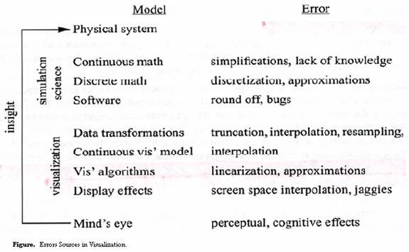
The first step in visualization study is to select a continuous mathematical model. Sometimes, we simplify the model because the problem is so complicated and we are lack of knowledge. The second step is to visualize the model in computer graphic system. In this step, we discretely sample the visualized object. Sometimes, we need to interpolate some data to get rid of artifact and jaggies after sampling. Surely, errors are introduced during this process because of simplification and interpolation.
In some field, these errors are very critical. For example, physician cannot compare tumor sizes which are measured at different stages in tumor diagnosis system if we cannot clarify the effects of errors in the final images. Different visualization algorithms have different errors and different fields can bear different degrees of errors. So we must have one way to compare all the 3D visualization algorithms. These results are precious for users to select a correct algorithm to visualize the dataset.
We live in a 3 dimensional physical world. So, a true 3D model can increase our insight of our world. For example, we all know that bio-polymers, such as protein, DNA and RNA etc., play important role in physiological activities of organisms. The 3D structure (high level structure) of these polymers is very crucial for their functions. If they lost their 3D structure, their bio-activity lost at the same time. So a lot of researches have been conducted to visualize the 3D structure of bio-polymers. This kind of 3D visualization is further being used to find the unknown high level structure of some bio-polymer based on the known 3D structure of some bio-polymers and the similarity of their low level structure. This application has already been used in pharmaceutical industrial to find new compounds, which possibly become a new drug [HMP98].
In general, volumetric comparison (the difference metrics) has the following usages [WU99]:
Well, we now know there must be errors in 3D visualization and it is important to know these errors qualitatively and quantitatively. Then the last question is how to compare two different volumetric rendering algorithms and derive the errors. There are two levels of comparison: image-based comparison and data-level comparison, which is illustrated in the following figure [KP99, PP94].
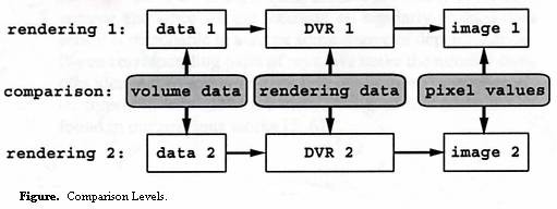
Image level comparison compares the final 3D images rendered by the different algorithms. Data level comparison does the comparison by using all the intermediate information during 3D rendering.
This method is simple and subjective. It provides users some final 3D images generated by different 3D rendering algorithms based on the same dataset. The users examine the difference with an overall assessment of the images. This method can tell the evident difference very easily. But its main drawback is that it leaves the burden to the users to identify regions of differences. Sometimes, these differences are very hard to tell, except the user is experienced or reminded by the people who generated these images. So, it is subjective and only qualitatively. This comparison only tells what the difference is, not how much difference is. So we should find some data to show how different images are.
There are some overall image statistical metrics, such as root-mean-square-error (RMSE), mean-absolute-error (MAE), peak signal-to-noise ratio, etc. Somebody also treat the images as a random function and calculate the statistical correlation p between two images. These metrics are defined as following:
MAE = ![]() ,
,
RMSE = ![]() ,
,
SNR =  ,
,
p(v, w) = ![]() =
= ![]() ,
,
where cov(v, w) is the covariance of the two random variables and s denotes standard deviations. The greater MAE and RMSE, the more different these two images are; SNR is on the contrary; the closer p is to 1, the more correlated are the two sample images.
The common feature of the above metrics is that they use the whole images as their starting point for comparison. It can tell the difference among images effectively and the difference is also comparable based on these metrics. However, it’s drawback is that it might obtain a small error sometimes, although the compared images look different.
The 2D difference image is another popular comparison method. The difference image is obtained by subtracting one image, B(i, j) from the other image, A(i, j). Then, the difference data of all the corresponding pixels are mapped to a grayscale value. If the two compared images are the same, the difference image should be all black. This method helps us to locate where the difference between two images is quickly. But, this method also has drawback. It is not effective when the difference between images is not very significant. In this case, we should use some image processing technique to stretch the contrast, such as histogram equalization.
This method is easily to extend to 3D data. We can use it to compare 3D datasets directly. I will talk about this in data level comparison part of this survey paper.
The main drawback of the above metrics and frequency domain metrics, which we will talk about below, is that they all do comparison based on the final 3D images. Therefore, a lot of 3D information is lost during calculations. Sometimes, this 3D information is valuable for comparing different algorithms. Data level comparison is such a comparison method, which makes use of intermediate and auxiliary information in the rendering process and uses this information to generate a data level comparison image. Of course, it is also not preclude the use of traditional methods such as side-by-side presentations when showing the results of the data level comparison. Currently, a lot of works that compared DVR algorithms by data level comparison have been published. The idea is illustrated in the following figure [KP99, KWP00]:
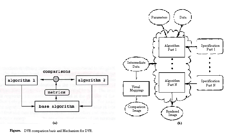
Normally data level comparison first needs to map other DVR algorithms to a base or reference algorithm, then collects the metrics from this base algorithm. The basic assumption in here is that the major differences among images, rendered by different DVR algorithms, result from those important rendering parameters, which we will talk about later in this paper. So we must specify all the rendering parameters and find the difference among these parameters, which results in the difference in final images. Projection-based DVR algorithms comparison and ray-based DVR algorithms comparison have been reported.
3D algorithms can also be compared in frequency domain instead of spatial domain. There are papers that use fast Fourier transformation and wavelet to do comparison. This technique is useful in distinguishing between low and high frequency signals and differences, as well as their orientations. There is an example in the Kwansik Kim’s paper, which shows the Fourier transforms of the three DVR images as well as their corresponding difference images.
N. Sahasrabudhe etc. [SWM99] proposed a complex spatial comparative metric. This metric is composed of 4 partial measures of differences between 2 images/datasets: (a) an overall or global point measure - M1, (b) a measure of the localization of differences or a lack of correlation – M2, (c) differences in areas of high transition or singularities and – M3, (d) areas of low transition or smoothness – M4. Not only does the complex metric let users find the magnitude of the difference, but also discern where the difference is located and whether the difference comes from high transition area or smooth area. These four partial metrics are defined as the following:
M1 =![]() ;
;
d(i, j) = A(i, j) – B(i, j);
m2(m, n) =![]() ;
;
r(m, n, k, l) = ![]() , where
, where
Al =![]() ; Bl =
; Bl = ; t is a parameter used to emphasize the
presence of difference, while de-emphasize their magnitude, in the
referred paper, t is equal to 0.25. r(m,n,k,l) is calculated over region
of pixels where (i,j) and (i+k,j+l) both lie in a ?x ? window centered
at (m,n).
; t is a parameter used to emphasize the
presence of difference, while de-emphasize their magnitude, in the
referred paper, t is equal to 0.25. r(m,n,k,l) is calculated over region
of pixels where (i,j) and (i+k,j+l) both lie in a ?x ? window centered
at (m,n).
M2 =![]() ;
;
Vh(i, j)=![]() ;
;
m3(i,j) = |d(i,j)|[Th((Vh(i,j)) + Tv(Vv(i,j)))];
M3 =![]() , where
, where
kh is the extent of the activity window at the horizontal direction, kv is at the vertical direction; Th and Tv are the threshold functions for selection of high transition areas.
M4 is calculated the same as M3, except they use different threshold functions. M4 is for areas of low transition areas.
One approach to compare different 3D rendering algorithms is to run these algorithms on standard test suites that, by general agreement, cover the important characteristics of certain classes of data. Different problem domains need different test suites. For example, computational fluid dynamics, geographical simulation and X-ray data present different challenges to visualization systems and therefore need different test datasets. Scientific data directly from experiments can be used as test datasets. But it is not sufficient. Scientific data are gathered for investigation, not for comparison. So, we must make up some standard algorithm comparison datasets to show the difference among algorithms. These datasets should be sensitive enough to the difference.
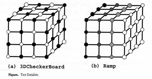
In Kwansik’s paper [KWP00, KWP01], 3DCheckerBoard and Ramp are used as test data sets. 3DCheckBoard is defined as:
V[I,
j, k] = ![]()
Here the voxels i, j, k over the domain [0...n-1], and take values of L (low) or H (high). Distance, d, is an integer that allows the checks to be d = 1, 2, 3, … in width in each dimension. The datasets are defined to be n x n x n in size. Ramp is defined as:
V[I, j, k] = L * (1-b) + H * b
Here the voxels I, j, k over the domain [0...n-1], and range from values of L (low) or H (high). These two test dataset are illustrated in the following figure [KWP00].
In P. Williams’ paper, the rendering parameter specifications are emphasized. In order to make an accurate comparison of images generated by different volume-rendering systems, a great care should be required in assuring that all the input and parameters (such as the scene, the viewing specification, the data set, etc.) are appropriately matched. Thus, a complete listing of all the input and parameters that require specification is an important pre-requisite for using any metrics.
He had an attempt to summarize a thorough list about these parameters [WU99]:
Data Set
Transfer Functions
Background
Lighting
Derived and Embedded Objects
Viewing Parameters
Optical Model
Image Specification
In general, there are three classes of differences: noise, bias and structured difference, each of which has a distinct perceptual impact. Noise is random or spurious differences in pixel values that are not part of any larger pattern. Sources of noise in a volume-rendered image can include: numerical or round-off error, stochastic sampling and numerical overflow during the computation of image. Bias is defined as a (relatively) uniform difference in intensity between images across the pixels of the image. Structured difference is that part of the aggregate difference image which consists of objects which have a coherent structural form, such as edges, haloes, lines, bright or dark spots, blobs, textures or any other patterns. The presence of structured difference means that the images being compared have a meaningful difference in content [WU99].
Noise can be filtered by using some image processing techniques (smoothing filters), such as neighbourhood averaging and lowpass filters. After we smooth the image, we can obtain the difference image between images before and after being filtered. This difference image is used to present noise at different location. Bias can be measured by using Median(A) – Median(B). So after noise and bias are got rid of from the total difference image, the resulting image is the structured difference image. An analysis of the structured difference image may yield important clues as to the source of the differences.
Comparative metrics in 3D rendering is not as old as 3D graphics. Working in this area is just starting. Additional work is needed on a wide variety of topics. For example, better understanding of catorgories of difference and metrics will improve the usefulness of the work; methods for analysing structured difference are application dependent and needs more carefully research; and wavelet metrics is a forthcoming hot point in this area... ...
[A03] Edward Angel, Interactive Computer Graphics: A Top-Down Approach Using OpenGL, 3rd edition, Addison-Wesley, c2003.
[GR94] Al Globus, Eric Raible, Fourteen Ways to Say Nothing with Scientific Visualization. IEEE Computers, vol. 27, no. 7 (July 1994), pp 86-88.
[GU95] Al Globus, Sam Uselton, Evaluation of Visualization Software. Report NAS-95-005, Feb. 1995.
[HMP98] Marc Hansen, Doanna Meads and Alex Pang, Comparative Visualization of Protein Structure-Sequence Alignments. IEEE Symposium on Information Visualization, October 19 - 20, 1998, North Carolina.
[KP99] Kwansik Kim, Alex Pang, A Methodology for Comparing Direct Volume Rendering Algorithms Using a Projection-based Data Level Approach. Proc. Eurographics/IEEE TVCG Symp. Visualization, pp. 87-98, May 1999.
[KP97] Kwansik Kim, Alex Pang, Ray-based Data Level Comparisons of Direct Volume Rendering Algorithms. Technical Report UCSC-CRL-97-15, UCSC Computer Science Department, 1997.
[KP01] Kwansik Kim, Alex Pang, Data Level Comparisons of Surface Classifications and Gradient Filters. Proceedings of Volume Graphics, May, 2001, Stony Brook, New York.
[KWP00] Kwansik Kim, Craig M.Wittenbrink, and Alex Pang, Maximal-Abstract Differences for Comparing Direct Volume Rendering Algorithms. April, 2000, Hewlett-Packard Laboratories Technical Report HPL-2000-40, also submitted to IEEE Transactions on Visualizations and Computer Graphics (TVCG).
[KWP01] Kwansik Kim, Craig M.Wittenbrink, and Alex Pang, Extended Specifications and Test Data Sets for Data Level Comparisons of Direct Volume Rendering Algorithms. IEEE Transactions on Visualization and Computer Graphics. Vol. 7, No. 4, Oct.-Dec., 2001.
[LZS02] Bill Lorensen, Karel Zulderveld, Vlkram Simha, Rainer Wegenkittl and Michael Meissner, Volume Rendering in Medical Applications: We’ve got pretty images, what’s left to do? IEEE Visualization 2002 Oct. 27 – Nov. 1, 2002.
[PP94] Hans-Georg Pagendarm, Frits H.Post, Comparative Visualization – Approaches and Examples. Fifth Eurographics Workshop on Visualization in Scientific Computing, Rostock, Germany, May 30 – June 1, 1994.
[SWM99] Nivedita Sahasrabudhe, John E.West, Raghu Machiraju, etc., Structured Spatial Domain Image and Data Comparison Metrics. In Proceedings of Visualization 99, p.97 – 104, 1999.
[T92] Lloyd Treinish, Correlative Data Analysis in the Earth Sciences, IEEE Computer Graphics & Applications, p.10 – 12, 1992.
[WU99] Peter L.Williams and Samuel P.Uselton, Metrics and Generation Specifications for Comparing Volume-rendered Images. J. Visual. Comput. Animat. 10, 159-178 (1999).
Prof. A. Pang’s group did some research on uncertainty visualization: http://www.cse.ucsc.edu/research/slvg/unvis.html;
Prof. R. Machiraju works on design of parametric studies using partial metrics: http://www.cis.ohio-state.edu/~raghu/;
NASA Vision Group: http://vision.arc.nasa.gov/.
This survey is based on electronic search in IEEE conference sites, IEEE homepage, and their digital libraries (www.computer.org and www.acm.org), "comparative 3D rendering algorithm" etc. used as keyword in search. Also, magazine of IEEE also searched, such as IEEE Communication Magazine.